Deep Learning with Torch¶

Credits: Soumith Chintala, Nicholas Leonard, Tyler Neylon, Adam Paszke

What is Torch?¶

Torch is a scientific computing framework based on Lua[JIT] with strong CPU and CUDA backends.

Strong points of Torch:

Efficient Tensor library (like NumPy) with an efficient CUDA backend
Neural Networks package -- build arbitrary acyclic computation graphs with automatic differentiation
- also with fast CUDA and CPU backends
Good community and industry support - several hundred community-built and maintained packages.

http://torch.ch
https://github.com/torch/torch7/wiki/Cheatsheet

Introduction - Lua¶

Lua is pretty close to javascript.
- variables are global by default, unless local keyword is used
Only has one data structure built-in, a table: {}. Doubles as a hash-table and an array.
1-based indexing.
foo:bar() is the same as foo.bar(foo)

Strings, numbers, tables¶

a = 'hello'

print(a)

b = {}

b[1] = a

print(b)

b[2] = 30

for i=1,#b do -- the # operator is the length operator in Lua (for LISTS ONLY)
    print(b[i])
end

If-Else¶

num = 40
if num == 40 then
  print('40')
elseif num ~= 40 then  -- ~= is not equals.
  print('not 40')
end

Functions¶

function fib(n)
  if n < 2 then return 1 end
  return fib(n - 2) + fib(n - 1)
end

-- Closures
function adder(x)
  -- The returned function is created when adder is
  -- called, and remembers the value of x:
  return function (y) return x + y end
end

Tables¶

a = {1, 2, ['a'] = 3}

a = {1, 2, a = 3, print = function(self) print(self) end}

a:print()

b = {1 = 'c'}

b

Metatables and Metamethods¶

Metatables allow us to change the behavior of a table. For instance, using metatables, we can define how Lua computes the expression a+b, where a and b are tables.
Values of __add, __index, ... are called metamethods.

f1 = {a = 1, b = 2}  -- Represents the fraction a/b.
f2 = {a = 2, b = 3}

metafraction = {}
function metafraction.__add(f1, f2)
  sum = {}
  sum.b = f1.b * f2.b
  sum.a = f1.a * f2.b + f2.a * f1.b
  return sum
end

setmetatable(f1, metafraction)

f1 + f2

-- An __index on a metatable overloads dot lookups
defaultFavs = {animal = 'gru', food = 'donuts'}
myFavs = {food = 'pizza'}
setmetatable(myFavs, {__index = defaultFavs})
print(myFavs.animal)

Direct table lookups that fail will retry using the metatable's __index value, and this recurses.

Classes¶

Classes aren't built in; there are different ways to make them using tables and metatables.

Dog = {}                                   -- 1.

function Dog.new()                         -- 2.
  newObj = {sound = 'woof'}                -- 3.
--   self.__index = self                      -- 4.
  return setmetatable(newObj, {__index = Dog})        -- 5.
end

function Dog:makeSound()                   -- 6.
  print('I say ' .. self.sound)
end

mrDog = Dog:new()                          -- 7.
-- mrDog['sound']
mrDog:makeSound()                          -- 8.
-- print(mrDog['sound'])

Dog acts like a class; it's really a table.
function tablename:fn(...) is the same as function tablename.fn(self, ...). The : just adds a first argument called self. Read 7 & 8 below for how self gets its value.
newObj will be an instance of class Dog.
self = the class being instantiated. Often self = Dog, but inheritance can change it. newObj gets self's functions when we set both newObj's metatable and self's __index to self.
Reminder: setmetatable returns its first arg.
The : works as in 2, but this time we expect self to be an instance instead of a class.
Same as Dog.new(Dog), so self = Dog in new().
Same as mrDog.makeSound(mrDog); self = mrDog.

Tensors¶

https://github.com/torch/torch7/blob/master/doc/tensor.md

Tensors are the main class of objects used in Torch 7:

An N-dimensional array that views an underlying Storage (a contiguous 1D-array)
Different Tensors can share the same Storage
Different types : FloatTensor, DoubleTensor, IntTensor, CudaTensor, and so on
Implements most Basic Linear Algebra Sub-routines (BLAS)
Supports random initialization, indexing, transposition, sub-tensor extractions, and more
Most operations for Float/Double are also implemented for Cuda Tensors (via cutorch)

a = torch.Tensor(5,3) -- construct a 5x3 matrix (initialized with garbage content, whatever was already there)

a = torch.rand(5,3)

print(a)

b=torch.rand(3,4)

print(b)

-- matrix-matrix multiplication: syntax 1
a*b

-- matrix-matrix multiplication: syntax 2
torch.mm(a,b)

-- matrix-matrix multiplication: syntax 3
c=torch.Tensor(5,4)
c:mm(a,b) -- store the result of a*b in c
print(c)

b = a
print(a)
print(b)

a:fill(1)

c = a:clone()
print(a)
print(c)

m = torch.Tensor(a:size()):copy(a)
print(m)

c:fill(1.8)
print(a)
print(c)

a = torch.Tensor(2, 3)

b = torch.Tensor(3, 2)

x = a:storage()
for i = 1, x:size() do
    x[i] = i
end

b[{{}, {1}}]:fill(2)
b[{{}, {2}}]:fill(3)

print(a)
print(b)

print(a*b)

CUDA Tensors¶

Tensors can be moved onto GPU using the :cuda function

require 'cutorch';
a = a:cuda()
b = b:cuda()
c = c:cuda()
c:mm(a,b) -- done on GPU

Transpose¶

a = torch.rand(5, 3)
print(a)

b = a:transpose(1, 2)
print(b)

Tensor a and b share the same underlying storage.

a[{2,1}] = 5
print(a)
print(b)

print(a:storage())
print(b:storage())

print(a:isContiguous())
print(b:isContiguous())

Neural Networks¶

Neural networks in Torch can be constructed using the nn package.

require 'nn';

implements feed-forward neural networks
neural networks form a computational flow-graph of transformations
backpropagation is gradient descent using the chain rule

For example, look at this network that classfies digit images: LeNet

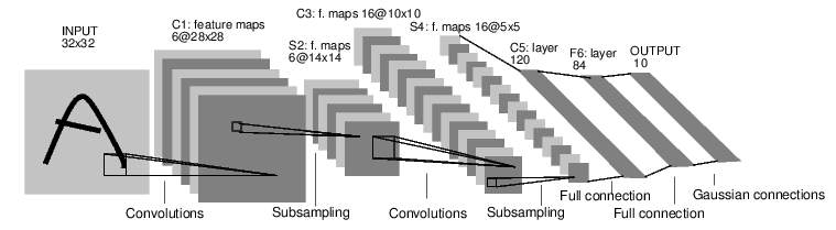
It is a simple feed-forward network. It takes the input, feeds it through several layers one after the other, and then finally gives the output.

Such a network container is nn.Sequential which feeds the input through several layers.

net = nn.Sequential()
net:add(nn.SpatialConvolution(1, 6, 5, 5)) -- 1 input image channel, 6 output channels, 5x5 convolution kernel
net:add(nn.SpatialMaxPooling(2,2,2,2))     -- A max-pooling operation that looks at 2x2 windows and finds the max.
net:add(nn.SpatialConvolution(6, 16, 5, 5))
net:add(nn.SpatialMaxPooling(2,2,2,2))
net:add(nn.View(16*5*5))                   -- reshapes from a 3D tensor of 16x5x5 into 1D tensor of 16*5*5
net:add(nn.Linear(16*5*5, 120))            -- fully connected layer (matrix multiplication between input and weights)
net:add(nn.Linear(120, 84))
net:add(nn.Linear(84, 10))                 -- 10 is the number of outputs of the network (in this case, 10 digits)
net:add(nn.LogSoftMax())                   -- converts the output to a log-probability. Useful for classification problems

print(net:__tostring());

mlp=nn.Parallel(2,1);     -- iterate over dimension 2 of input
mlp:add(nn.Linear(10,3)); -- apply to first slice
mlp:add(nn.Linear(10,2))  -- apply to first second slice
x = torch.randn(10,2)
print(x)
print(mlp:forward(x))

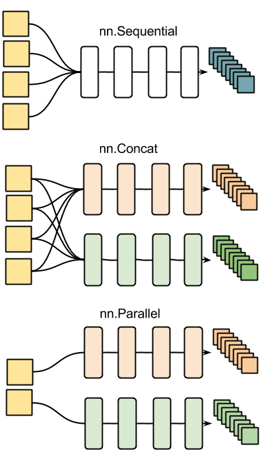
Other examples of nn containers are shown in the figure below:

Every neural network module in torch has automatic differentiation. It has a :forward(input) function that computes the output for a given input, flowing the input through the network. and it has a :backward(input, gradient) function that will differentiate each neuron in the network w.r.t. the gradient that is passed in. This is done via the chain rule.

input = torch.rand(1,32,32) -- pass a random tensor as input to the network

output = net:forward(input)

net:zeroGradParameters() -- zero the internal gradient buffers of the network (will come to this later)

gradInput = net:backward(input, torch.rand(10))

print(#gradInput)

Criterion: Defining a loss function¶

When you want a model to learn to do something, you give it feedback on how well it is doing. This function that computes an objective measure of the model's performance is called a loss function.

A typical loss function takes in the model's output and the groundtruth and computes a value that quantifies the model's performance.

The model then corrects itself to have a smaller loss.

In torch, loss functions are implemented just like neural network modules, and have automatic differentiation.
They have two functions - forward(input, target), backward(input, target)

For example:

criterion = nn.ClassNLLCriterion() -- a negative log-likelihood criterion for multi-class classification

loss = criterion:forward(output, 3) -- let's say the groundtruth was class number: 3

gradients = criterion:backward(output, 3)

gradInput = net:backward(input, gradients)

Training¶

require 'optim';

Optimization package for nn.
Provides training algorithms like SGD, LBFGS, etc.
Uses closures

parameters, gradParameters = net:getParameters()

-- Define a closure that computes the loss and dloss/dx.
feval = function(x)
    -- reset gradients
    gradParameters:zero()

    -- 1. compute outputs (log probabilities) for each data point
    local output = net:forward(input)
    -- 2. compute the loss of these outputs, measured against the true labels
    local loss = criterion:forward(output, 3)
    -- 3. compute the derivative of the loss wrt the outputs of the model
    local dloss_doutput = criterion:backward(output, 3)
    -- 4. use gradients to update weights
    net:backward(input, dloss_doutput)

    -- optim expects us to return
    -- loss, (gradient of loss with respect to the weights)
    return loss, gradParameters
end

-- Define SGD parameters.
sgd_params = {
    learningRate = 1e-2,
    learningRateDecay = 1e-4,
    weightDecay = 0,
    momentum = 0
}

-- train for a number of epochs
epochs = 1e2
losses = {}
for i = 1,epochs do
    -- one step of SGD optimization (steepest descent)
    _,local_loss = optim.sgd(feval, parameters, sgd_params)
    -- accumulate error
    losses[#losses + 1] = local_loss[1]
end
print(losses[1])
print(losses[#losses])

print(torch.exp(net:forward(input)))

Network graphs¶

https://github.com/torch/nngraph

nngraph provides graphical computation for the nn library in Torch.

require 'nngraph';

nngraph overloads the call operator (i.e. the () operator used for function calls) on all nn.Module objects.
When the call operator is invoked, it converts the nn.Module to nngraph.gModule.
The argument to the call operator specifies which modules will feed into this one during a forward pass.

add = nn.CAddTable()
t1 = torch.Tensor{1,2,3}
t2 = torch.Tensor{4,5,6}
output = add:forward({t1, t2})

print(t1 + t2)

x1 = nn.Identity()()
x2 = nn.Identity()()
a = nn.CAddTable()({x1, x2})
m = nn.gModule({x1, x2}, {a})

print(m:forward{t1, t2})

Vanilla RNN¶

input_size = 3
rnn_size = 2

inputs = {}
table.insert(inputs, nn.Identity()()) -- network input
table.insert(inputs, nn.Identity()()) -- h at time t-1
input = inputs[1]
prev_h = inputs[2]

i2h = nn.Linear(input_size, rnn_size)(input) -- input to hidden
h2h = nn.Linear(rnn_size, rnn_size)(prev_h)  -- hidden to hidden

next_h = nn.Tanh()(nn.CAddTable(){i2h, h2h})

outputs = {}
table.insert(outputs, next_h)

-- packs the graph into a convenient module with standard API (:forward(), :backward())
RNN = nn.gModule(inputs, outputs)

print(RNN:forward{torch.randn(1,3), torch.randn(1,2)})

print(RNN:backward({torch.Tensor{0,0,0}, torch.Tensor{0,0}}, torch.randn(1,2)))

RNN:get(1)

LSTM Implementation¶

http://apaszke.github.io/lstm-explained.html
http://colah.github.io/posts/2015-08-Understanding-LSTMs/

Gates:

$$ i_t = g(W_{xi}x_t + W_{hi}h_{t-1} + b_i) $$$$ f_t = g(W_{xf}x_t + W_{hf}h_{t-1} + b_f) $$$$ o_t = g(W_{xo}x_t + W_{ho}h_{t-1} + b_o) $$

Input transform:

$$ c\_in_t = tanh{(W_{xc}x_t + W_{hc}h_{t-1} + b_c)} $$

State update:

$$ c_t = f_t ⋅ c_{t-1} + i_t ⋅ c\_in_t $$$$ h_t = o_t ⋅ tanh{(c_t)} $$

input_size = 3
rnn_size = 2

inputs = {}
table.insert(inputs, nn.Identity()())   -- network input
table.insert(inputs, nn.Identity()())   -- c at time t-1
table.insert(inputs, nn.Identity()())   -- h at time t-1
input = inputs[1]
prev_c = inputs[2]
prev_h = inputs[3]

$$ i_t = g(W_{xi}x_t + W_{hi}h_{t-1} + b_i) $$$$ f_t = g(W_{xf}x_t + W_{hf}h_{t-1} + b_f) $$$$ o_t = g(W_{xo}x_t + W_{ho}h_{t-1} + b_o) $$$$ c\_in_t = tanh{(W_{xc}x_t + W_{hc}h_{t-1} + b_c)} $$

i2h = nn.Linear(input_size, 4 * rnn_size)(input)  -- input to hidden
h2h = nn.Linear(rnn_size, 4 * rnn_size)(prev_h)   -- hidden to hidden
preactivations = nn.CAddTable()({i2h, h2h})       -- i2h + h2h

All the gates use the sigmoid, and the input preactivation uses tanh.

-- gates
pre_sigmoid_chunk = nn.Narrow(2, 1, 3 * rnn_size)(preactivations)
all_gates = nn.Sigmoid()(pre_sigmoid_chunk)

-- input
in_chunk = nn.Narrow(2, 3 * rnn_size + 1, rnn_size)(preactivations)
in_transform = nn.Tanh()(in_chunk)

in_gate = nn.Narrow(2, 1, rnn_size)(all_gates)
forget_gate = nn.Narrow(2, rnn_size + 1, rnn_size)(all_gates)
out_gate = nn.Narrow(2, 2 * rnn_size + 1, rnn_size)(all_gates)

Cell and Hidden states

$$ c_t = f_t ⋅ c_{t-1} + i_t ⋅ c\_in_t $$$$ h_t = o_t ⋅ tanh{(c_t)} $$

-- previous cell state contribution
c_forget = nn.CMulTable()({forget_gate, prev_c})
-- input contribution
c_input = nn.CMulTable()({in_gate, in_transform})
-- next cell state
next_c = nn.CAddTable()({c_forget, c_input})

c_transform = nn.Tanh()(next_c)
next_h = nn.CMulTable()({out_gate, c_transform})

Defining the module

-- module outputs
outputs = {}
table.insert(outputs, next_c)
table.insert(outputs, next_h)

-- packs the graph into a convenient module with standard API (:forward(), :backward())
LSTM = nn.gModule(inputs, outputs)

print(LSTM:forward{torch.randn(1,3):zero(), torch.randn(1,2):zero(), torch.randn(1,2):zero()})

print(LSTM:backward({torch.randn(1,3), torch.randn(1,2), torch.randn(1,2)}, {torch.randn(1,2):zero(), torch.randn(1,2):zero()}))

LSTM.modules

Where do I go next?¶

Build crazy graphs of networks: https://github.com/torch/nngraph
Train on imagenet with multiple GPUs: https://github.com/soumith/imagenet-multiGPU.torch
Train recurrent networks with LSTM on text: https://github.com/wojzaremba/lstm
More demos and tutorials: https://github.com/torch/torch7/wiki/Cheatsheet
Chat with developers of Torch: http://gitter.im/torch/torch7
Ask for help: http://groups.google.com/forum/#!forum/torch7